Archive for May 2011
Closed-form solution of modified Ornstein-Uhlenbeck process
Process definition
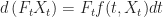
In this article we deduce the closed-from solution of the modified version of Ornstein-Uhlenbeck process:
where 


Integrating factor approach
There exists a general approach to non-linear stochastic differential equations of the form:
where 


The method consists of:
- Define the integrating factor:
- So the original equation could be written as
- Now define
so that - And it yields the deterministic differential equation for each


We can therefore solve it with 


Calibration of Ornstein-Uhlenbeck process
Introduction
In mathematics, Ornstein-Uhlenbeck process satisfies the following stochastic differential equation:
where

In finance, it is used to model interest rates, currency exchange rates and commodity prices. Although it is usually modified to incorporate non-negativity of prices.
Ordinary Least-Squares Approach to calibration
The simplest approach to the calibration problem is to convert SDE to finite difference equation (as it is usually used in Monte Carlo simulation) and to rearrange parts to Ordinary Least Squares equation.
The simplest updating formula for Ornstein-Uhlenbeck process is:
By rearranging we obtain:
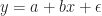
Comparing with simple regression formula:
we can equate as follows:
and immediately obtain the following:


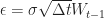


As 
where 


So, regression of 

The modified process
Let’s consider the process with slight modification and apply the same approach to the modified process:
Then the naive updating formula is
Then dividing by
Given simple regression formula:
we can equate as follows:
and immediately obtain the following:
Applying the same logic as in previous section, finally we get:


Therefore, regression of 

Open questions
- Bias of the estimators. For the original process this approach usually gives quite precise estimation of mean and volatility but fails to provide mean reversion parameter
- Closed-form solution of the modified SDE. It could be used to improve the updating formula
- Statistical hypothesis testing if the sample drawn from the process. This is quite crucial point as it helps to identify model regime shift in trading.

